I first stumbled upon hooks when I was trying to implement CheferCAM during my internship for the explainability of ViTs. This is how a code snippet from that codebase look like. It was kind of very strange to me, at that time.
def forward_hook(self, input, output):
    if type(input[0]) in (list, tuple):
        self.X = []
        for i in input[0]:
            x = i.detach()
            x.requires_grad = True
            self.X.append(x)
    else:
        self.X = input[0].detach()
        self.X.requires_grad = True

    self.Y = output


def backward_hook(self, grad_input, grad_output):
    self.grad_input = grad_input
    self.grad_output = grad_output
I got to know that Hooks is one of the most powerful yet under-documented features in PyTorch. When working with complex deep learning models—especially “black box” architectures like Vision Transformers (ViTs)—we often need to peek inside to understand how information flows.
Before we dive into Hooks, there’s one prerequisite. Hooks allow us to dynamically interrupt the computational graph in the forward or backward pass. If “static” and “dynamic” computational graphs are alien to you, I strongly suggest you to read this amazing post about computational graphs.
Whether you are debugging a model, working on interpretability, or trying to visualize what a specific layer is focusing on, you need access to intermediate outputs. Modifying the source code of a library (like timm or torchvision) to return these values is messy and unsustainable.
This is where PyTorch Hooks come in. They allow you to dynamically inspect internal module inputs and outputs during the forward or backward pass without altering the model definition.
In this post, I will demonstrate how to use forward hooks to extract activations and attention maps from a Vision Transformer (vit_tiny_patch16_224) available in the timm library.
1. Setting Up the Environment
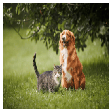
First, let’s load the necessary libraries and a sample image. We will use a pre-trained ViT model.
import torch
import timm
from PIL import Image
import numpy as np
import matplotlib.pyplot as plt
from collections import OrderedDict
import torch.nn.functional as F
import math

# Load a sample image (ensure you have an image path ready)
dog_img_path = "Sample Images/dog_image.png"
dog_img_np = np.array(Image.open(dog_image.png))

# Preprocessing function
def preprocess_img(img_np):
    img = torch.from_numpy(img_np).permute(2,0,1).float() / 255.0
    img = F.interpolate(img.unsqueeze(0), size=(224,224),
                        mode='bilinear', align_corners=False).squeeze(0)

    mean = torch.tensor([0.485, 0.456, 0.406]).view(3,1,1)
    std  = torch.tensor([0.229, 0.224, 0.225]).view(3,1,1)

    img = (img - mean) / std
    return img

dog_img_tensor = preprocess_img(dog_img_np)
Original Image
2. Loading the Model
We will use the vit_tiny_patch16_224 model. It is small enough to run quickly but complex enough to demonstrate the utility of hooks.
model = timm.create_model("vit_tiny_patch16_224.augreg_in21k_ft_in1k", pretrained=True)
model.eval()
3. Capturing Activations using Hooks
To capture the output of each Transformer block, we need to register a “forward hook.” A forward hook is a function that is executed every time the specific layer performs a forward pass.
We will store the outputs in an OrderedDict and keep track of the hook handles so we can remove them later.
activations_od = OrderedDict()
hook_handles = []

def get_activations(name:str):
  def activation_hook(module, input, output):
    activations_od[name] = output.detach()
  return activation_hook

# Add hooks to all the blocks to capture layer-wise activations
for i, block in enumerate(model._modules['blocks']):
  h = block.register_forward_hook(get_activations(f"block_{i}"))
  hook_handles.append(h)
4. Capturing Attention Maps
Capturing attention maps in optimized libraries like timm can be tricky. Modern implementations often use F.scaled_dot_product_attention (Flash Attention) or fuse operations for speed, meaning the raw Attention Map () is never explicitly materialized as a tensor we can grab.
To solve this, we can capture the Query (Q) and Key (K) embeddings separately and manually reconstruct the attention map.
First, we must ensure fused attention is disabled if possible, or hook into the normalization layers preceding the attention calculation.
# Create storage for Q and K
attention_maps_od = OrderedDict()
q_embeddings_od = OrderedDict()
k_embeddings_od = OrderedDict()

# Hook functions
def get_query_activations(name:str, q_scale:float):
  def query_activation_hook(module, input, output):
    # We apply the scale here to match the implementation logic
    q_embeddings_od[name] = output.detach() * q_scale
  return query_activation_hook

def get_key_activations(name:str):
  def key_activation_hook(module, input, output):
    k_embeddings_od[name] = output.detach()
  return key_activation_hook

# Register hooks on the Q_norm and K_norm layers inside the Attention block
for i, block in enumerate(model._modules['blocks']):
  attn_block = block._modules['attn']

  # Hooks for Q and K
  h1 = attn_block.q_norm.register_forward_hook(get_query_activations(f"block_{i}", attn_block.scale))
  h2 = attn_block.k_norm.register_forward_hook(get_key_activations(f"block_{i}"))
  hook_handles.append(h1)
  hook_handles.append(h2)
Now, we need a trigger to actually compute . Since the MLP block always runs after the Attention block, we can register a hook on the MLP block to compute the attention map using the Q and K we just captured.
def get_attention_maps(name:str):
  def compute_attn_map_hook(module, input, output):
    q = q_embeddings_od[name]
    k = k_embeddings_od[name]

    # Calculate Attention Map
    attn = q @ k.transpose(-2, -1)
    attention_maps_od[name] = attn.softmax(dim=-1)

  return compute_attn_map_hook

# Register the trigger hook on the MLP block
for i, block in enumerate(model._modules['blocks']):
  mlp_block = block._modules['mlp']
  h = mlp_block.register_forward_hook(get_attention_maps(f"block_{i}"))
  hook_handles.append(h)
5. Running Inference
Now that our hooks are set, we simply pass the image through the model. The hooks will automatically populate our dictionaries.
x = dog_img_tensor.unsqueeze(0)
with torch.inference_mode():
  output = model(x)
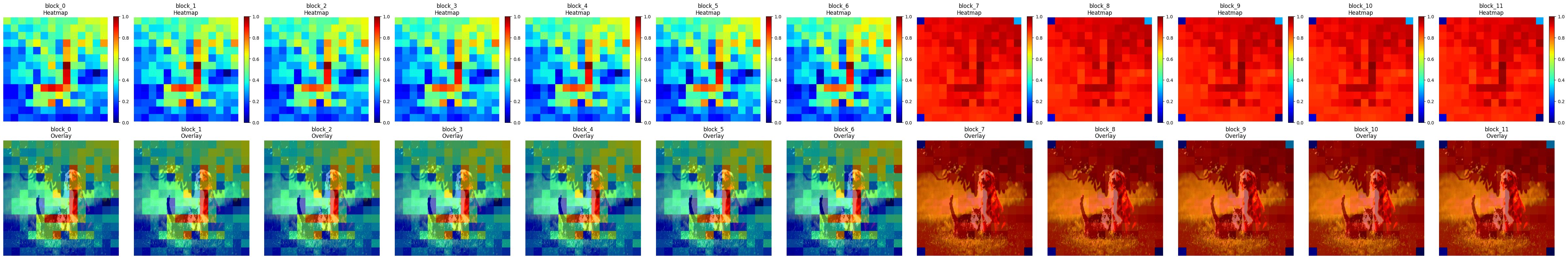
6. Visualizing Activations
Let’s visualize the raw activations. The output of a ViT block is a sequence of tokens. To visualize this as an image, we remove the [CLS] token, take the mean across the feature dimension, and reshape the remaining patch tokens back into a 2D grid (14x14).
# Visualize activations across all layers
def visualize_all_layers(x, activations_od, normalized=True, alpha=0.5, cmap='jet', interpolation='bilinear'):
    if x.dim() == 4: x = x[0]

    # Denormalize image for display
    if normalized:
        mean = torch.tensor([0.485, 0.456, 0.406]).view(3,1,1)
        std  = torch.tensor([0.229, 0.224, 0.225]).view(3,1,1)
        x = x * std + mean
    img = x.permute(1, 2, 0).clamp(0, 1).cpu().numpy()

    num_layers = len(activations_od)
    fig, axes = plt.subplots(2, num_layers, figsize=(4 * num_layers, 8))

    for idx, (layer_name, activation_tensor) in enumerate(activations_od.items()):
        # Remove [CLS] and take mean
        activation_patches = activation_tensor.squeeze(0)[1:, :].mean(dim=-1)

        # Reshape to grid
        NUM_PATCHES = int(math.sqrt(activation_patches.shape[0]))
        activation_grid = activation_patches.view(NUM_PATCHES, NUM_PATCHES)

        # Upsample
        activation_map = activation_grid.unsqueeze(0).unsqueeze(0)
        mode = 'nearest' if interpolation == 'nearest' else 'bilinear'
        activation_resized = F.interpolate(activation_map, size=(224, 224), mode=mode).squeeze()

        # Normalize to [0, 1] for visualization
        act = activation_resized.cpu().numpy()
        act = (act - act.min()) / (act.max() - act.min() + 1e-8)

        # Plot Heatmap
        axes[0, idx].imshow(act, cmap=cmap)
        axes[0, idx].axis('off')
        axes[0, idx].set_title(f'{layer_name}')

        # Plot Overlay
        axes[1, idx].imshow(img)
        axes[1, idx].imshow(act, cmap=cmap, alpha=alpha)
        axes[1, idx].axis('off')

    plt.tight_layout()
    plt.show()

visualize_all_layers(x, activations_od, normalized=False, alpha=0.6, interpolation='nearest')
Activation Maps Propogation over the layers
7. Visualizing Attention Maps
Finally, let’s visualize the Attention Maps. Specifically, we are looking at how the [CLS] token attends to the image patches. This gives us an idea of what the model considers “important” for classification at each layer.
def visualize_attention_grid(x, attention_maps_od, slice_idx=0, normalized=True, alpha=0.6, cmap='jet'):
    x_img = x[0]
    if normalized:
        mean = torch.tensor([0.485, 0.456, 0.406]).view(3, 1, 1)
        std = torch.tensor([0.229, 0.224, 0.225]).view(3, 1, 1)
        x_img = x_img * std + mean
    img = x_img.permute(1, 2, 0).clamp(0, 1).cpu().numpy()

    num_layers = len(attention_maps_od)
    fig, axes = plt.subplots(2, num_layers, figsize=(4*num_layers, 8))

    for col, (layer_name, attn_tensor) in enumerate(attention_maps_od.items()):
        # Average over heads, take CLS token's attention to patches
        attn_slice = attn_tensor.squeeze(0).mean(dim=0)[slice_idx, 1:]

        # Reshape and Upsample
        N = int((attn_slice.shape[0])**0.5)
        attn_map = attn_slice.view(1, 1, N, N)
        attn_resized = F.interpolate(attn_map, size=(224, 224), mode='nearest').squeeze().cpu().numpy()

        # Plot
        axes[0, col].imshow(attn_resized, cmap=cmap)
        axes[0, col].axis('off')
        axes[0, col].set_title(f'{layer_name}')

        axes[1, col].imshow(img)
        axes[1, col].imshow(attn_resized, cmap=cmap, alpha=alpha)
        axes[1, col].axis('off')

    plt.tight_layout()
    plt.show()

visualize_attention_grid(x, attention_maps_od, slice_idx=0)
Attention Maps Propogation over the layers
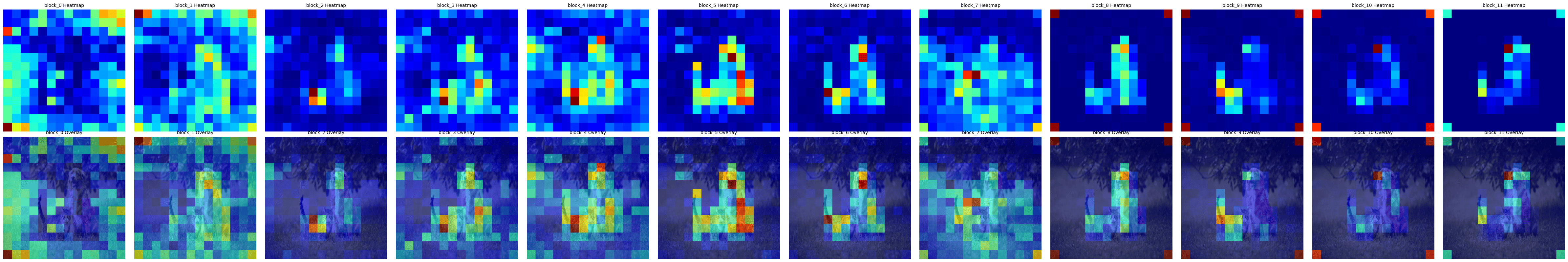
EDIT: Now, you might be wondering what has happened after the 8th layer, why there’s a drastic difference in the attention maps? I wrote about this phenomenon in my blog post “How I Stumbled Upon a major Vision Transformer Flaw (and Found the Fix)”.
Conclusion
Using PyTorch Hooks, we successfully extracted internal states from a ViT model without altering its source code. We saw how the model’s focus changes layer by layer—activations generally show feature responses, while attention maps reveal how the model aggregates information to the [CLS] token. This technique is essential for model interpretability and research.
Don’t forget to clean up your hooks when you are done!
for h in hook_handles:
    h.remove()
8. References
-
PyTorch 101, Understanding Graphs, Automatic Differentiation and Autograd https://www.digitalocean.com/community/tutorials/pytorch-101-understanding-graphs-and-automatic-differentiation
-
PyTorch 101: Understanding Hooks https://www.digitalocean.com/community/tutorials/pytorch-hooks-gradient-clipping-debugging
-
CheferCAM Codebase https://github.com/hila-chefer/Transformer-Explainability
-
PyTorch Hooks Explained - In-depth Tutorial https://www.youtube.com/watch?v=syLFCVYua6Q
-
Visualizing activations with forward hooks (PyTorch) https://www.youtube.com/watch?v=1ZbLA7ofasY