SASIKA
AMARASINGHE
Final-year Electronic & Telecommunication Engineering undergraduate at University of Moratuwa, Sri Lanka.
Focusing on Spatio-Temporal 3D Visual Grounding on Dynamic Point Clouds, advised by Dr. Ranga Rodrigo, and Dr. Vigneshwaran Subbaraju.
Passionate about Computer Vision, Multimodal Learning, and Embodied AI.


Publications
-
FreqPAC: Frequency-based Preference-guided Adaptation of Attentional Features for Compact Vision-Language Models
Under Review -
CL4D: Contrastive Language–4D Pretraining for Zero-Shot Action-to-Text Retrieval and 4D Large Language Models
Under Review
Experience & Updates
Research Intern (Remote)
Jul 2025 - PresentA*STAR Institute of High Performance Computing (IHPC) 🇸🇬
- Conducting research on Spatio-Temporal 3D Visual Grounding on Dynamic Point Clouds.
Research Intern
Dec 2024 - Jun 2025Singapore Management University & M3S, SMART Lab 🇸🇬
- Engineered a preference-guided optimization pipeline integrating feedback from frontier models to fine-tune attention maps. Applied this to Preference-Guided Few-Shot Adaptation and Grounded Planning for embodied agents (inspired by LLM-Planner).
- Output: Co-authored manuscript FreqPAC: Frequency-based, Preference-Guided, Few-Shot Adaptation of Compact Models Using Human Feedback Augmented By AI (Under revision).
Webmaster
Dec 2024 - Dec 2025IEEE Signal Processing Society Student Branch Chapter, UoM
Honorary Mention - Team QSentinel
Nov 2024IEEE ComSoc Student Competition 2024
- ⭐️ Our project LOTEN and LOTUDP: Enhancing Secure, Reliable, Real-Time Communication for IoT Devices in Critical Applications received a Honorary mention at IEEE ComSoc Student Competition 2024.
Winner - Team EcoNova
Sep 2024Spark Challenge 2024, UoM
- 🥇 First Place Winner of this Sustainability Challenge out of all the teams from Electronics and Telecommunication Engineering Department.
- Pitched EcoNova Agri-Voltaic Solar Project.
- Received a grant worth 600,000 LKR to work on our pilot project.
Winner - Team QSentinel
Aug 2024ComFix 2024, IEEE ComSoc UoM
- 🥇 Pitched Qsentinal IOT Suite for this communication based competition.
Writing
-
The Cost of Being Wrong: KL Divergence
-
Capture Activations and Attention Maps using PyTorch Hooks
-
From Telecom Lectures to Deep Learning: Finally Understanding Entropy
-
A guide for the unkown: #ScholarX
-
Enhancing Low Light Images: A Deep Dive into Autoencoders
-
Hybrid Images through Frequency Wizardry
Projects

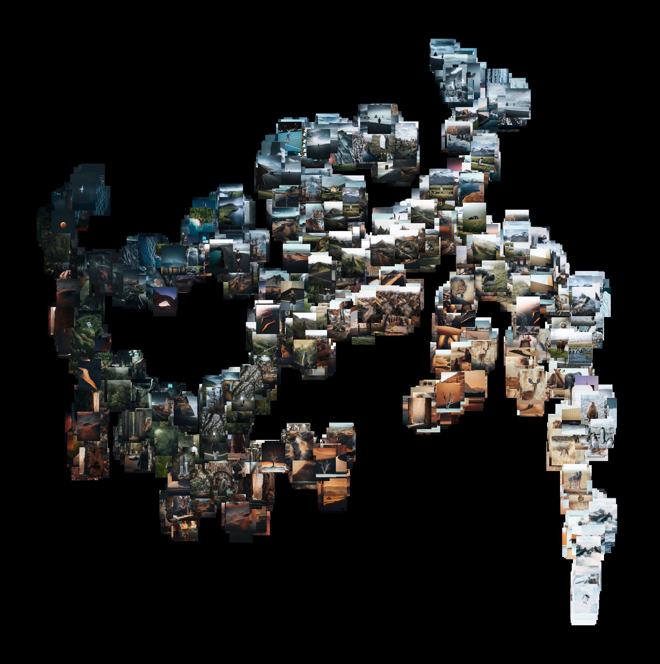
🔮 Mapping Photography Portfolios by Visual Similarity With Machine Learning
I scraped the profile of @withluke and created these visualizations optimized to load around 2250 images. Click to see the live demo.
The methods used were inspired by:
- 3D View — Google Arts Experiments TSNE Viewer
- Spherical View — IsoMatch: Creating Informative Grid Layouts
- Grid View — IsoMatch: Creating Informative Grid Layouts
Prior to this, I built a Python implementation, which you can find here: Grid-Layout-Image-Artwork. This pipeline can be replicated for any image dataset (including any Instagram profile) to create a grid layout using PCA or non-linear dimensionality reduction methods such as t-SNE or UMAP.

👁️ Evaluation Tool for Vision Encoder Explainability Methods
A tool to evaluate different explainability methods for Vision Transformer Architectures. Deployed in 🤗 HuggingFace Spaces
We created this tool to evaluate different explainability methods for different Vision Transformer Architectures:
- LeGrad (ICCV 2025 – to be implemented)
- CheferCAM (CVPR 2021)
- Attention Rollout (ACL 2020)
- Grad-CAM (IJCV 2019)
You can perturb the image (+ ve/ - ve) and see how it affects the final prediction.
Supported model families include ViT, DeiT, DinoV2, and ViTs with Registers (ICLR 2024).
You can check the live demo here: Hugging Face Space

🚶 3D Human Trajectory Tracking in Point Clouds using a Standard Kalman Filter
Implementation of Kalman Filter for tracking humans using 3D point cloud data.
This project focuses on implementing state estimation to track a human subject within a dynamic point cloud environment. Developed for the Autonomous Systems module and inspired by research into 4D Visual Grounding, the system employs a Standard Kalman Filter (KF) under a Constant Velocity motion model. A critical component of the measurement model is the Sonata (Point Transformer v3) neural network. In this pipeline, the Sonata model is responsible for segmenting the human subject from the larger point cloud scene, allowing the system to extract the centroid $(x, y, z)$ as the measurement vector.

🧠 Embodied AI: Low-Resource Cross-Architecture Knowledge Transfer for Vision-Language Models
This is the work that I did during my internship at SMU & M3S.
The following document is a brief summary of some of the work I did during my internship. Note that it does not comprise the work to the fullest extent.
GitHub - https://github.com/a073-vlm-onedge
Project Report

🌐 Jetson-Hololens Distributed Server Integration
Engineered a distributed system connecting an NVIDIA Jetson (Edge), Microsoft HoloLens 2, and a remote server for hybrid inference. Developed a pipeline where visual and audio inputs from the HoloLens are processed by lightweight VLM (Moondream, Florence-2) on the Jetson or offloaded to large VLM(Llama 3.2 Vision) on the remote server.
- Engineered a distributed system connecting an NVIDIA Jetson (Edge), Microsoft HoloLens 2, and a remote server for hybrid inference.
- Developed a pipeline where visual and audio inputs from the HoloLens are processed by lightweight VLM (Moondream, Florence-2) on the Jetson or offloaded to large VLM(Llama 3.2 Vision) on the remote server.

💡 iCliQ
A wearable clicker for public speakers and professionals, created by our team, 'Company of Noobs' for the Engineering Design Project in Semester 2. I was responsible for developing the firmware. This project helped us reach the final rounds of several hackathons.

iCliQ is a a wearable clicker for public speakers and other professionals, developed by our team Comany of Noobs for the EN1190 : Engineering Design Project module in Semester 2 at the Electronic and Telecom. Engineering - University of Moratuwa.
All the design files (Altium and Solidworks files), code, documentation, user manual is available in github repository
This project provided us with a great opportunity to engage in different stages of electronic product development from ideation, prototyping to commercialization. In this journey we had to learn many aspects of product design regarding idea validation, market analysis and many more. Also we acquired many technical skills such as PCB designing, enclosure designing, embedded UI designing and prototyping.
🔆 iCliQ
iCliQ is a novel wearable clicker powered by ESP32 WROOM SoC featuring;
- ✅ A 4-layer PCB to improve EMI performance and achieve a compact design
- ✅ Generating vibrational haptic patterns at specific time intervals
- ✅ RGB LED based visual indicator to embed the time card concept.
- ✅ Simple and fast pairing with any device using Bluetooth LE 4.2
- ✅ Enabling seamless control of presentation tools (Powerpoint, Canva)
- ✅ Precisely timing speeches and presentations
- ✅ Red color laser pointer visible up to 20 meters.
- ✅ Compatible with Windows, MacOS and Android devices
- ✅ Incorporating an intuitive ergonomic design
- ✅ A modern embedded user interface.
- ✅ Rechargable battery with battery life up to 6 hours
- ✅ Fast charging


🔆 Identified Issue:
Both professional and amateur speakers often face challenges when it comes to managing their time during speeches or presentations, regardless of whether they are delivering a short-prepared speech or a long impromptu speech or pitching a presentation. Short-prepared speeches can be particularly challenging, as speakers may have difficulty staying on schedule without the aid of time cards or a clock. Additionally, for longer speeches such as keynotes or lectures, it’s crucial to adhere to specific timing to keep the audience engaged and prevent the presentation from becoming boring.
🔆 Hardware Specifications:
- ESP32
- OLED display
- Bluetooth Low Energy (BLE) 4.2
- Surface-mount device (SMD) soldering
🔆 Software Tools Used :
- Altium
- SolidWorks
- VS Code
🔆 Future Scope:
-
Research and Development in to provide more accessibility features for users with special needs to help them become better public speakers.
-
Applying for industrial design.
-
We have already applied for a short-term fund from “AHEAD” program of World Bank through UBLC to manufacture a small batch for testing and pilot projects.
🔆 The Team - Company of Noobs
Our project was selected for the finals of HackX 2023 Inter-University Startup Challenge organized by University of Kelaniya.


🤖🦾 Computer Vision System for Industrial Bin Picking Robot Arm
Computer Vision System for Bin Picking Task using image Segmentation models such as SAM, DeepLab, Unet, Segnet and attempt to implement in an industrial robot arm
In this project, our assigned task was to build a computer vision system to get the coordinates of a single box given an image using a segmentation method.
This task is a simplified version of Bin Picking which is a core problem in computer vision and robotics.
DeepLab Model
In this first attempt, the team along with my group mate, Isiri Withanawasam was asked to refer to Semantic Segmentation model : DeepLab paper and implement the model for our application.
Since the DeepLab model is not trained on any segmentation dataset which contains box images, a dataset of about 100 annotated images is created.


Then the DeepLabV3 model was trained on our custom dataset using transfer learning. This is the result we got after 25 epochs.

Since we were not satisfied with the results, we found the paper SAM model and moved onto using it according to the advice by our supervisor.
SAM Model
Using this model (Segment Anything by MetaAI), we could get the desired output we were looking for. The results were taken in Google Colab using a NVIDIA Tesla T4 GPU.


Fast SAM Model
Since we want a real time inference of the model, and our computation to happen on an edge device. Therefore we wanted to use the model with Fast SAM. With this model we could get the result even in edge with less time using CPU compared to the SAM model sacrifising some accuracy and gaining advantage of inference time.
On Local Machine

On Raspberry PI 4B

Note : The image in Raspberry Pi is not shown because, Ubuntu Server was running in the Raspberry Pi 4B with no GUI. That is the reason for QT error.
Camera integration & Multithreading
To decrease the time for inference we use multithreading to get input imags from the camera in one thread and buffer them. And do the computation in another thread to get the output. See the latest commit in old branch in the github repository. (not yet merged to main branch)
Future Improvements
By the time I am writing this, we have successfully completed the assigned task. As part of the hardware project we have created a custom gripper.
After the evaluation day, we hope to integrate this vision system and the custom gripper with an industrial robot arm using ROS2, going the extra mile.
We have already checked two robot arms available in our university’s Electrical Engineering Department. Here are those robot arms.


Specifications of the above robot arms

📃 GCE AL 2020 Student Performance Dataset
Created a dataset of results of candidates who sat for GCE AL (University Entrance Examination) containing more than 330,000 records
🌐 Kaggle Link
This dataset contains information on the performance of students in the GCE Advanced Level (AL) exam in Sri Lanka in 2020. It was collected by Sasika Amarasinghe and is available on Kaggle.
I have removed some columns of the original dataset due to ethical reasons. But here’s a sample of the data when a search query is given.
Dataset Characteristics
- The dataset consists of over 300,000 records of student performance in the GCE AL exam in Sri Lanka.
- The data includes information on student identification, school, district, medium of instruction, stream, and their scores in different subjects.
- The data also includes the overall Z-score of each student, which is a standard score that indicates the number of standard deviations by which the student’s exam results are above or below the mean.
Variables
-
Index: A unique identifier for each student -
School ID: Identification number of the school -
District: District where the school is located -
Stream: Science, Arts, or Commerce stream of the student -
Medium: Sinhala or English medium of instruction -
Subjects: The scores of the student in each of the subjects - Mathematics, Science, English, Buddhism, and History -
Z-Score: The overall Z-score of the student
Use Cases
- This dataset can be used to study the performance of students in different subjects and in different streams, medium of instruction, and districts.
- The data can also be used to study the relationship between student performance and demographic factors such as medium of instruction and district.
- This dataset can be used to identify the factors that contribute to the performance of students in the GCE AL exam and to make recommendations for improving student performance in the future.
Usability
- 9.41 / 10
Sources
- Data were collected from (https://www.doenets.lk/examresults) which is the exam result site in Sri Lanka
Collection Methodology
- Data were scraped data by a python script written by the author using the index no as the key.
- Later the national identity card numbers were decoded to extract applicants’ birthdays and gender.
- For privacy concerns, “Full name”,”National Identity Card no” and “Index no” were removed, but the birthdays and genders have been added to the dataset.
- Used AWS instances to collect data parallely to reduce the time and data usage.
I got a bronze 🥉 medal for this dataset with 36 upvotes in the Kaggle Community. and very good feedback from the Community Members.
Testimonials for the dataset
⭐ This can be actually used to look after the academic likelihoods and whereabouts of Sri Lankan students’ academics! Great job! – VISHESH THAKUR - Datasets Expert
⭐ This data could be used for EDA, visualization and even model development! Good work and great dataset! – RAVI RAMAKRISHNAN-Notebooks Grandmaster
Github Link
I haven’t publicized the code for the datascraping and datapreprocessing,search queries of students. Not available due to ethical reasons.

🎥 Real-Time 4K Video Exposure Correction Pipeline
Extended WACV 2024 implementation for real-time 4K video exposure correction.
- Extended the official WACV 2024 implementation of “4K-Resolution Photo Exposure Correction” (~8K params) from static image processing to a full video inference pipeline.
- Engineered a frame-buffering mechanism to handle 4K input streams, optimizing GPU VRAM usage.
- Implemented frame-wise inference logic to enable rapid exposure correction on video data.
🔮 t-SNE visualizer for image data
Converts any image dataset into 2D t-SNE visualization
t-SNE is a powerful technique for visualizing high-dimensional data in a low-dimensional space. It is particularly useful for exploring the structure of complex datasets and identifying patterns or clusters.
This repository contains a Python package for visualizing high-dimensional data using t-distributed Stochastic Neighbor Embedding (t-SNE) algorithm.
Features
- Apply t-SNE to your high-dimensional data (especially image datasets).
- Visualize the results in 2D.
- Customize the visualization with various parameters
- Save the visualizations as image files.
Gallery


References
[1] L.J.P. van der Maaten and G.E. Hinton, "Visualizing High-Dimensional Data Using t-SNE," Journal of Machine Learning Research, vol. 9, pp. 2579-2605, 2008. [Online]. Available: https://www.jmlr.org/papers/volume9/vandermaaten08a/vandermaaten08a.pdf
[2] G.E. Hinton and R.R. Salakhutdinov, "Reducing the Dimensionality of Data with Neural Networks," Science, vol. 313, no. 5786, pp. 504-507, 2006. [Online]. Available: https://www.cs.toronto.edu/~hinton/absps/tsne.pdf

🔆 D2BGAN
PyTorch Implementation of paper titled D2BGAN: A Dark to Bright Image Conversion Model for Quality Enhancement and Analysis Tasks Without Paired Supervision
D2BGAN Model Implementation from scratch

![]()
Paper
D2BGAN: A Dark to Bright Image Conversion Model for Quality Enhancement and Analysis Tasks Without Paired Supervision
Summary of D2BGAN paper
D2BGAN is a CycleGAN model that is designed to convert low light images to bright images. It is an unpaired GAN-based image enhancement operation that uses cycle consistency, geometric consistency, and illumination consistency. The model has been shown to provide competitive results on standard benchmark datasets, and it has been observed to perform well on DICM, LIME, and MEF datasets when D2BGAN was applied. However, it does not perform well on backlit images.
Difference between conventional CycleGAN and D2BGAN
In conventional CycleGAN 2 generators and 2 discriminators have been used. However, in D2BGAN architecture, 2 generators and 8 discriminators have been used.
In D2BGAN , in each domain, 4 discriminators have been used (8 discriminators altogether)
- color discriminator 1
- color discriminator 2
- RGB images with 2 blurred factors are passed through these 2 discriminators
- texture discriminator
- A grayscale of an image was used for this discriminator
- edge discriminator
- The edge image which was obtained by Prewitt operator (any edge filter will do) to pass through this discriminator
For the loss, compared to conventional CycleGAN , in addition to Adversarial Loss and Cycle Loss, a new loss “consistency loss” has been introduced which represent geomentric consistency and illumination consistency.
The idea of illumination consistency is supported by the fact that two same low light images with slightly different illumination can generate the same enhanced image. The network is guided to a single translation at a time, thereby controlling the open-ended nature of the problem to some extent. in addition, the generalization capability of the network is improved, and false structure generation is reduced.
The geometric consistency acts in a similar fashion and ensures that the false data generation tendency of the generator is checked.
These two consistencies consider the structure and illumination factors of the image, improving the overall illumination without saturation while preserving the structure at the same time.
To set up the geometric and lighting consistency constraints, we transform X(image in X domain) into X_g and X_l, where X_g is a 90-degree rotation of X and X_l is a gamma transformation of X.
Gamma transformation (correction) is a non-linear operation used to encode and decode luminance or tristimulus values in still image systems.


References

🤖 Bots
Automated bots for Instagram and Twitter using Selenium (Python)
🔰 Instagram Bot

🌐 Github repo
This is an Instagram bot written in Python that automates several tasks on Instagram, including logging in, sending messages, and chatting with other users.
Key Features
- Automated login to Instagram using provided credentials
- Ability to send messages to specified users over specific time intervals
- Ability to chat with other users when given their Instagram URL
The bot is designed to make it easier to manage multiple Instagram accounts and automate repetitive tasks. It leverages the power of Python programming to simplify these tasks and streamline the Instagram experience.
Getting Started
To use this repository, you will need to have a basic understanding of Python programming and be familiar with using the terminal. Before you get started, make sure you have the necessary dependencies installed, including the latest version of Python.
If you have any questions or run into any issues, please feel free to open an issue in the repository or reach out to the repository owner for support.
NOTE: Currently, this repository is not under development.
🔰 Twitter Bot
🌐 Github repo
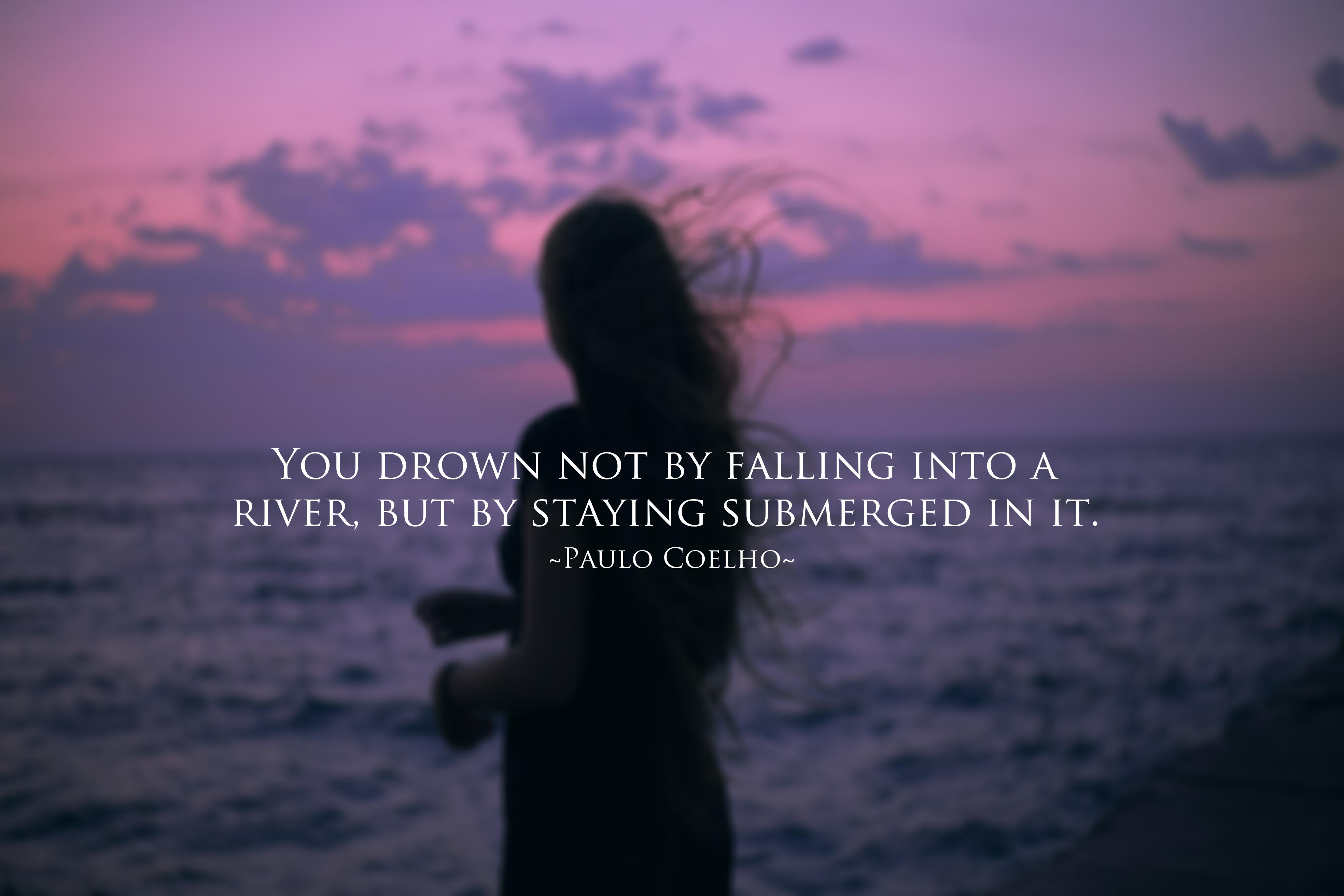
This Twitter bot is designed to fetch quotes from an API, retrieve images from a stock image site, process the image, and post it to Twitter. The bot is written in Python using the Selenium library and is capable of tweeting at specific intervals over a duration of time.
Here is my Twitter automated profile that I maintained using this Twitter bot:
Key Features
- Fetches quotes from an API
- Retrieves images from a stock image site
- Processes the image to enhance its visual appeal
- Posts the quote and image to Twitter at specific intervals
- Written in Python using the Selenium library
Getting Started
- Clone the repository to your local machine.
- Install the required libraries specified in the
requirements.txtfile. - Provide your Twitter API credentials in the designated fields in the code.
- Run the script and watch as the bot posts quotes and images to Twitter at the specified intervals.
Support
For support and questions, please open an issue in the repository or reach out to the repository owner.
Enjoy tweeting quotes and images with this Twitter bot!
NOTE: This repository is not currently under development.

🫂 Unilink Project - Social media platform
A full stack webapp for community building developed using Django. This can be used for boilerplate for building any community
This is a social media project that is developed using Django Framework as backend. Our main goal of this project was to build a platform to connect with other university students. This has similar funcionalities like other Social Media Platforms like Facebook.
🌐 Github repo
Here’s my 🌐blog article related to this project.
UniLink Project
Funcionalities available so far in the site :
- User Signup
- User Login/Logout
- (Django Inbuilt user authentication)
- Password Reset ( Using Twillio as a service )
- News Feed similar to Facebook (not yet user oriented so far)
- Make posts and edit them
- User Authorization features
This is how to get started and customize it.
1) First, clone the repository.
git clone https://github.com/SasikaA073/Social-blog
2) Then run this command to activate a python environment. After that activate the environment.
In linux,

    virtualenv --python=python3 ~/venv/MyVirtEnv
    source ~/venv/MyVirtEnv/bin/activate

In Windows,

    python -m venv "MyVirtEnv"
    source MyVirtEnv\Scripts\activate

If your Python virtual environment works fine, then in the command line should be something similar to this.


    (MyVirtEnv) C:\Users\Foo
3) Now you have to install the required python libraries. Then run this command.
pip install -r requirements.txt
4) Now the last part!
python manage.py runserver
Technologies Used
- Python (Django framework)
- SQLite (Database management system)
Credits
developed by: Sasika Amarasinghe Hasitha Gallella
Guidance by: Damsith Adikari Chamika Jayasinghe Yasaara Weerasinghe


🔊 MFCC Speaker Recognition
Audio Signal Processing Challenge 2024 on Robovox Dataset for far-field speaker recognition by a mobile robot
I worked with audio signal data for in this challenge (Signal Processing Cup 2024 organized by IEEE Signal Processing Society). Here is some overview what we have done in this project.


This repository contains files related to the Signal Processing Cup 2024 competition by Team EigenSharks.
Contents
Folders
Denoising
This folder contains the code for the denoising task using Matlab and Python implementations. Continuous Wavelet Transform has been used for denoising.

Explore Dataset
This folder contains the code for exploring the dataset. The code is written in Python and uses the librosa library for audio processing. The code is divided into two main files: explore_dataset.py and explore_dataset.ipynb. The former is a Python script that can be run from the command line, while the latter is a Jupyter notebook that can be run interactively.
Feature Extraction
This folder contains the code for extracting features from the audio files.
The following figure shows the architecture of the x-vector model used for feature extraction:

-
paper - Xvector Paper
-
from_scratch.ipynb - Extract features from the noisy audio files
-
from_scratch_denoised_version.ipynb = Extract features from the denoised audio files
-
avg_xvectors_from_scratch_densoised_version.ipynb - Extract features from the denoised audio files using the average of the x-vectors for each speaker
-
English_xvector_from_scratch_denoised_version.ipynb - Extract features from the denoised audio files using SpeechBrain’s pretrained x-vector model
-
Transfer Learning Jtubespeech.ipynb - Use transfer learning to train JtubeSpeech’s x-vector model on the denoised French Audio dataset
French Audio Generation
French_Audio_Generation.ipynb contains code for synthesizing French audio using Google Text-to-Speech and pyttsx3.
Speaker recognition
I_go_from_scratch.ipynb contains code for attempt to train a speaker recognition model from scratch using Triplet Loss.
Submissions
fourth_submission.zip - This gave the best result on the leaderboard. from_scratch_denoised_version.ipynb was used to generate the submission file.
submission_template.py - A python script to generate the submission file, by simply changing the model architecture.

Problem Statement : RoboVox: Far-field speaker recognition by a mobile robot
Introduction
A speaker recognition system authenticates the identity of claimed users from a speech utterance. For a given speech segment called enrollment and a speech segment from a claimed user, the speaker recognition system will determine automatically whether both segments belong to the same speaker or not. The state-of-the-art speaker recognition systems mainly use deep neural networks to extract speaker discriminant features called speaker embeddings.
The DNN-based speaker verification systems perform well in general, but there are some challenges that reduce their performance dramatically. Far-field speaker recognition is among the well-known challenges facing speaker recognition systems. The far-field challenge is intertwined with other variabilities such as noise and reverberation. Two main categories of speaker recognition systems are text-dependent speaker recognition vs text-independent speaker recognition. In a text-dependent speaker recognition system, the speaker’s voice is recorded from predefined phrases, while, in text-independent speaker recognition, there is no constraint on the content of the spoken dialogue. The task of the IEEE Signal Processing Cup 2024 is text-independent far-filed speaker recognition under noise and reverberation for a mobile robot.
Task description
The Robovox challenge is concerned with doing far-field speaker verification from speech signals recorded by a mobile robot at variable distances in the presence of noise and reverberation. Although there are some benchmarks in this domain such as VoiCes and FFSVC, they don’t cover variabilities in the domain of robotics such as the robot’s internal noise and the angle between the speaker and the robot. The VoiCes dataset is replayed speech recorded under different acoustical noises. A main drawback of the VoiCes is that it was recorded from played signals whereas our dataset is recorded with people speaking in noisy environments. The FFSVC is another far-field speaker recognition benchmark. However, these benchmarks helped the community significantly, we are introducing a new benchmark for far-field speaker recognition systems in order to address some new aspects. Firstly, our goal is to perform speaker recognition in a real application for the domain of mobile robots. In this domain, there are other variabilities that have not been addressed in previous benchmarks: the robot’s internal noise and the angle between the speaker and the robot. Furthermore, the speech signal has been recorded for different distances between the speaker and the robot. In the proposed challenge the following variabilities are present:
- Ambient noise leading to low signal-to-noise ratios (SNR): The speech signal is distorted with noise from fans, air conditioners, heaters, computers, etc.
- Internal robot noises (robot activators): The robot’s activator noise reverberates on the audio sensors and degrades the SNR.
- Reverberation: The phenomena of reverberation due to the configuration of the places where the robot is located. The robot is used in different rooms with different surface textures and different room shapes and sizes.
- Distance: The distance between the robot and speakers is not fixed and it is possible for the robot to move during the recognition.
- Babble noise: The potential presence of several speakers speaking simultaneously.
- Angle: The angle between speakers and the robot’s microphones
Robovox tasks
In this challenge, two tracks will be proposed:
-
Far-field single-channel tracks: In this task, one channel is used to perform the speaker verification. The main objective is to propose novel robust speaker recognition pipelines to tackle the problem of far-field speaker recognition in the presence of reverberation and noise.
-
Far-field multi-channel tracks: In this task, several channels are used to perform speaker verification. The main objective is to develop algorithms that improve the performance of multi-channel speaker verification systems under severe noise and reverberation.
References
[1] - D. Snyder, D. Garcia-Romero, G. Sell, D. Povey, and S. Khudanpur, “X-vectors: Robust DNN embeddings for speaker recognition,” in 2018 IEEE International Conference on Acoustics, Speech and Signal Processing (ICASSP), Calgary, AB, Canada, 2018, pp. 5329-5333. [Online]. Available: https://www.danielpovey.com/files/2018_icassp_xvectors.pdf

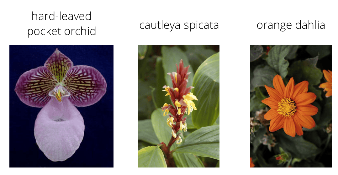
🌸 Flower Images Classifier
Finetuned model with backbone of VGG16 & Resnet to classify 102 classes of flower images. Deployed in 🤗 Hugging Face Spaces
This is my final project in the AI programming with Python Nanodegree program by Udacity. You can find the complete project repository here.
🌐 Github Link
This project consists of two parts.
- Jupyter Notebook part
- Command line application to predict the class of a flower once the image is given.
- In this article I have changed the content from the original Jupyter Notebook file.
In this project, I have trained an image classifier to recognize different species of flowers. I used this dataset of 102 flower categories. These are some examples.
The project is broken down into multiple steps:
- Load and preprocess the image dataset
- Train the image classifier on your dataset
- Use the trained classifier to predict image content
# Imports packages
import torch
from torch import nn, optim
import torch.nn.functional as F
from torchvision import datasets, transforms, models

import numpy as np
import pandas as pd

import seaborn as sb
import matplotlib.pyplot as plt

from PIL import Image

import time,json

%matplotlib inline
%config InlineBackend.figure_format = 'retina'
Load the data
The dataset is split into three parts, training, validation, and testing. For the training, it is required to use transformations such as random scaling, cropping, and flipping. This will help the network generalize leading to better performance. Make sure data is resized to 224x224 pixels as required by the pre-trained networks.
The validation and testing sets are used to measure the model’s performance on data it hasn’t seen yet.
The pre-trained networks you’ll use were trained on the ImageNet dataset where each color channel was normalized separately. For all three sets you’ll need to normalize the means and standard deviations of the images to what the network expects. For the means, it’s [0.485, 0.456, 0.406] and for the standard deviations [0.229, 0.224, 0.225], calculated from the ImageNet images. These values will shift each color channel to be centered at 0 and range from -1 to 1.
data_dir = 'flowers'
train_dir = data_dir + '/train'
valid_dir = data_dir + '/valid'
test_dir = data_dir + '/test'

# Define your transforms for the training, validation, and testing sets
train_transforms = transforms.Compose([transforms.RandomRotation(30),
                                       transforms.RandomResizedCrop(224),
                                       transforms.RandomHorizontalFlip(),
                                       transforms.RandomVerticalFlip(),
                                       transforms.ToTensor(),
                                       transforms.Normalize([0.485, 0.456, 0.406],
                                                            [0.229, 0.224, 0.225])])

test_valid_transforms = transforms.Compose([transforms.Resize(255),
                                            transforms.CenterCrop(224),
                                            transforms.ToTensor(),
                                            transforms.Normalize([0.485, 0.456, 0.406],
                                                                 [0.229, 0.224, 0.225])])
# Load the datasets with ImageFolder
train_data = datasets.ImageFolder(train_dir, transform=train_transforms)
valid_data = datasets.ImageFolder(valid_dir, transform=test_valid_transforms)
test_data = datasets.ImageFolder(test_dir, transform=test_valid_transforms)

# Using the image datasets and the trainforms, define the dataloaders
train_loader = torch.utils.data.DataLoader(
    train_data, batch_size=32, shuffle=True)
valid_loader = torch.utils.data.DataLoader(
    valid_data, batch_size=32, shuffle=True)
test_loader = torch.utils.data.DataLoader(test_data, batch_size=32)
Label mapping
Loads a json file, and convert it into a dictionary mapping the integer encoded categories to the actual names of the flowers.
with open('cat_to_name.json', 'r') as f:
    cat_to_name = json.load(f)

cat_to_name

output_layer_size = len(cat_to_name)
Building and training the classifier
# Build and train your network
model = models.densenet201(pretrained=True)

# To view the model architecture
model
    Downloading: "https://download.pytorch.org/models/densenet201-c1103571.pth" to /root/.torch/models/densenet201-c1103571.pth
    100%|██████████| 81131730/81131730 [00:01<00:00, 64976186.49it/s]

    DenseNet(
      (features): Sequential(
        (conv0): Conv2d(3, 64, kernel_size=(7, 7), stride=(2, 2), padding=(3, 3), bias=False)
        (norm0): BatchNorm2d(64, eps=1e-05, momentum=0.1, affine=True, track_running_stats=True)
        (relu0): ReLU(inplace)
        (pool0): MaxPool2d(kernel_size=3, stride=2, padding=1, dilation=1, ceil_mode=False)
        (denseblock1): _DenseBlock(
          (denselayer1): _DenseLayer(
            (norm1): BatchNorm2d(64, eps=1e-05, momentum=0.1, affine=True, track_running_stats=True)
            (relu1): ReLU(inplace)
            (conv1): Conv2d(64, 128, kernel_size=(1, 1), stride=(1, 1), bias=False)
            (norm2): BatchNorm2d(128, eps=1e-05, momentum=0.1, affine=True, track_running_stats=True)
            (relu2): ReLU(inplace)
            (conv2): Conv2d(128, 32, kernel_size=(3, 3), stride=(1, 1), padding=(1, 1), bias=False)
          )
          ...
          ...
          ...
          (denselayer30): _DenseLayer(
            (norm1): BatchNorm2d(1824, eps=1e-05, momentum=0.1, affine=True, track_running_stats=True)
            (relu1): ReLU(inplace)
            (conv1): Conv2d(1824, 128, kernel_size=(1, 1), stride=(1, 1), bias=False)
            (norm2): BatchNorm2d(128, eps=1e-05, momentum=0.1, affine=True, track_running_stats=True)
            (relu2): ReLU(inplace)
            (conv2): Conv2d(128, 32, kernel_size=(3, 3), stride=(1, 1), padding=(1, 1), bias=False)
          )
          (denselayer31): _DenseLayer(
            (norm1): BatchNorm2d(1856, eps=1e-05, momentum=0.1, affine=True, track_running_stats=True)
            (relu1): ReLU(inplace)
            (conv1): Conv2d(1856, 128, kernel_size=(1, 1), stride=(1, 1), bias=False)
            (norm2): BatchNorm2d(128, eps=1e-05, momentum=0.1, affine=True, track_running_stats=True)
            (relu2): ReLU(inplace)
            (conv2): Conv2d(128, 32, kernel_size=(3, 3), stride=(1, 1), padding=(1, 1), bias=False)
          )
          (denselayer32): _DenseLayer(
            (norm1): BatchNorm2d(1888, eps=1e-05, momentum=0.1, affine=True, track_running_stats=True)
            (relu1): ReLU(inplace)
            (conv1): Conv2d(1888, 128, kernel_size=(1, 1), stride=(1, 1), bias=False)
            (norm2): BatchNorm2d(128, eps=1e-05, momentum=0.1, affine=True, track_running_stats=True)
            (relu2): ReLU(inplace)
            (conv2): Conv2d(128, 32, kernel_size=(3, 3), stride=(1, 1), padding=(1, 1), bias=False)
          )
        )
        (norm5): BatchNorm2d(1920, eps=1e-05, momentum=0.1, affine=True, track_running_stats=True)
      )
      (classifier): Linear(in_features=1920, out_features=1000, bias=True)
    )


```python
input_layer_size = model.classifier.in_features
output_layer_size = len(cat_to_name)
class FlowerClassifier(nn.Module):

    """
    Fully connected / Dense network to be used in the transfered model
    """

    def __init__(self, input_size, output_size, hidden_layers, dropout_p=0.3):
        """
        Parameters
        ----------

            input_size : no of units in the input layer (usually the pretrained classifier's
            features_in value)

            output_size : no of units (no of classes that we have to classify the dataset)

            hidden_layers : a list with no of units in each hidden layer

            dropout_p : dropout probability (to avoid overfitting)

        """

        super().__init__()

        self.hidden_layers = nn.ModuleList(
            [nn.Linear(input_size, hidden_layers[0])])

        layer_sizes = zip(hidden_layers[:-1], hidden_layers[1:])
        self.hidden_layers.extend([nn.Linear(h1, h2)
                                  for h1, h2 in layer_sizes])

        self.output = nn.Linear(hidden_layers[-1], output_size)

        # add a dropout propability to avoid overfitting
        self.dropout = nn.Dropout(p=dropout_p)

    def forward(self, x):

        for each in self.hidden_layers:
            x = self.dropout(F.relu(each(x)))

        x = self.output(x)
        x = F.log_softmax(x, dim=1)

        return x
# Use GPU for computaion if it's available
device = torch.device("cuda" if torch.cuda.is_available() else "cpu");
# funtion to train the model
def train(model, epochs, criterion, optimizer, train_loader=train_loader, valid_loader=valid_loader, manual_seed=42):
    """
        Train the given model.


        Parameters
        ----------
        model : model for the classification problem

        epochs : no of complete iterations over the entire dataset

        criterion : loss function / cost function to see how much our model has been deviated from the real values
                examples :: Categorical Cross-Entropy Loss , Negative Log-Likelihood Loss

        optimizer : The algorithm that is used to update the parameters of the model
                examples :: Stochastic Gradient Descent (SGD) , Adam algorithm

        train_loader : loader for the training dataset

        valid_loader : loader fot the validation dataset


        Returns
        -------
        performance_list : a list with details of the model during each epoch

    """

    performance_list = []

    torch.manual_seed(manual_seed)

    start = time.time()

    with active_session():

        for e in range(1,epochs+1):

            train_total_loss = 0
            valid_total_loss = 0

            for images, labels in train_loader:

                # move images and labels data from GPU to CPU, back and forth.
                images = images.to(device)
                labels = labels.to(device)

                log_ps = model(images)
                loss = criterion(log_ps, labels)
                train_total_loss += loss.item()

                # To avoid accumulating gradients
                optimizer.zero_grad()

                # Back propagation
                loss.backward()
                optimizer.step()

            model.eval()

            accuracy = 0

            with torch.no_grad():
                for images, labels in valid_loader:

                    images = images.to(device)
                    labels = labels.to(device)


                    log_ps = model.forward(images)
                    loss = criterion(log_ps, labels)
                    valid_total_loss += loss.item()

                    top_p, top_class = log_ps.topk(1)
                    equals = top_class == labels.view(*top_class.shape)
                    accuracy += 100 * torch.mean(equals.type(torch.FloatTensor)).item()

                accuracy = accuracy / len(valid_loader)
                train_loss = train_total_loss / len(train_loader)
                valid_loss = valid_total_loss / len(valid_loader)

                performance_list.append((e , train_loss, valid_loss, accuracy, model.state_dict()))

                end = time.time()
                epoch_duration = end - start
                print(f"Epoch: {e}, Train loss: {train_loss:.3f}, Valid loss: {valid_loss:.3f}, Accuracy: {accuracy:.3f}%, time duration per epoch: {epoch_duration:.3f}s")

            model.train()

    return performance_list

# function to test the model performance
def validation(model, criterion, test_loader, device):

    """"
    Test the performance of the model on a test dataset

    Parameters
    ----------
        model : model for the classification problem

        criterion : loss function / cost function to see how much our model has been deviated from the real values
            examples :: Categorical Cross-Entropy Loss , Negative Log-Likelihood Loss

        test_loader : loader fot the test dataset

        device : use `gpu` or `cpu` for computation

    Returns
    ----------
        a tuple with the accuracy and test_loss on the given dataset


    """

    model.eval()
    model.to(device)
    accuracy = 0

    with torch.no_grad():
        test_loss = 0
        for images, labels in test_loader:

            images = images.to(device)
            labels = labels.to(device)

            log_ps = model.forward(images)

            test_loss += criterion(log_ps, labels).item()

            top_p, top_class = log_ps.topk(1, dim=1)
            equals = top_class == labels.view(*top_class.shape)
            accuracy += 100 * (torch.mean(equals.type(torch.FloatTensor)).item())

        test_loss = test_loss / len(valid_loader)
        accuracy = accuracy / len(valid_loader)


        print(f"Accuracy: {accuracy:.3f}%\nTest loss: {test_loss:.3f}")
        return (accuracy, test_loss)
model = models.densenet201(pretrained=True)

# Freeze parameters so we don't backprop through them
for param in model.parameters():
    param.requires_grad = False

hidden_layer_units = [1024, 512, 256]
my_classifier = FlowerClassifier(input_layer_size, output_layer_size, hidden_layer_units, dropout_p=0.2)
model.classifier = my_classifier

model.to(device)

optimizer = optim.Adam(model.classifier.parameters(), lr=0.003)
criterion = nn.NLLLoss()

model_list = train(model=model, epochs=16, optimizer=optimizer, criterion=criterion)
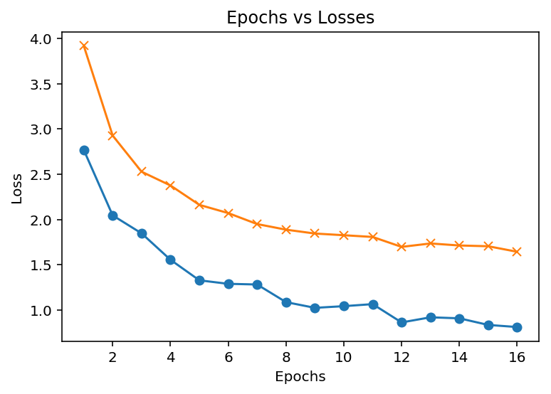
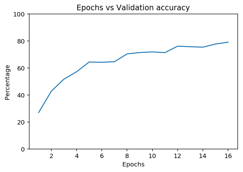
    Epoch: 1, Train loss: 3.917, Valid loss: 2.767, Accuracy: 26.976%, time duration per epoch: 194.214s
    Epoch: 2, Train loss: 2.926, Valid loss: 2.045, Accuracy: 42.762%, time duration per epoch: 376.733s
    Epoch: 3, Train loss: 2.527, Valid loss: 1.847, Accuracy: 51.656%, time duration per epoch: 559.668s
    Epoch: 4, Train loss: 2.376, Valid loss: 1.555, Accuracy: 57.118%, time duration per epoch: 742.296s
    Epoch: 5, Train loss: 2.161, Valid loss: 1.328, Accuracy: 64.370%, time duration per epoch: 924.386s
    Epoch: 6, Train loss: 2.070, Valid loss: 1.289, Accuracy: 64.156%, time duration per epoch: 1106.762s
    Epoch: 7, Train loss: 1.949, Valid loss: 1.282, Accuracy: 64.557%, time duration per epoch: 1289.242s
    Epoch: 8, Train loss: 1.887, Valid loss: 1.087, Accuracy: 70.353%, time duration per epoch: 1471.411s
    Epoch: 9, Train loss: 1.845, Valid loss: 1.024, Accuracy: 71.381%, time duration per epoch: 1653.647s
    Epoch: 10, Train loss: 1.826, Valid loss: 1.042, Accuracy: 71.822%, time duration per epoch: 1835.788s
    Epoch: 11, Train loss: 1.807, Valid loss: 1.065, Accuracy: 71.314%, time duration per epoch: 2017.690s
    Epoch: 12, Train loss: 1.697, Valid loss: 0.863, Accuracy: 76.068%, time duration per epoch: 2199.950s
    Epoch: 13, Train loss: 1.735, Valid loss: 0.919, Accuracy: 75.681%, time duration per epoch: 2381.585s
    Epoch: 14, Train loss: 1.713, Valid loss: 0.908, Accuracy: 75.347%, time duration per epoch: 2563.224s
    Epoch: 15, Train loss: 1.704, Valid loss: 0.835, Accuracy: 77.658%, time duration per epoch: 2745.755s
    Epoch: 16, Train loss: 1.643, Valid loss: 0.812, Accuracy: 79.046%, time duration per epoch: 2927.450s
# dataframe to store performance of the model, so that we can change the hyperparameters
model_performance_architecture_df = pd.DataFrame(model_list)
model_performance_architecture_df.rename(
    columns={
        0: 'epoch',
        1: 'train_loss',
        2: 'valid_loss',
        3: 'valid_accuracy',
        4: 'state_dict'
    },inplace=True)

model_performance_df = model_performance_architecture_df.iloc[:, :4]
plt.plot(model_performance_df['epoch'], model_performance_df['valid_loss'],'-o',label='validation loss')
plt.plot(model_performance_df['epoch'], model_performance_df['train_loss'], '-x', label='training loss');

plt.xlabel('Epochs')
plt.ylabel('Loss')
plt.title('Epochs vs Losses');
plt.plot(model_performance_df['epoch'], model_performance_df['valid_accuracy'])
plt.xlabel('Epochs')
plt.ylabel('Percentage')
plt.title("Epochs vs Validation accuracy")

plt.ylim(0, 100);
Testing the network
The network is tested on the images that the network has never seen either in training or validation. This gives a good estimate for the model’s performance on completely new images.
# Do validation on the test set
validation(model, nn.NLLLoss(), test_loader, 'cuda');
Accuracy: 79.194%
Test loss: 0.832
Save the checkpoint
Here after the network is trained, it is saved in oreder to load it later for making predictions.
Make sure to include any information that is needed in the checkpoint, to rebuild the model for inference. It is necessary to include pretrained network architecture as well. Otherwise conflicts can be happened.
# Save the checkpoint
checkpoint = {'input_size' : input_layer_size,
             'output_size' : output_layer_size,
             'hidden_layers' : [each.out_features for each in model.classifier.hidden_layers],
             'model_data' : pd.DataFrame(model_list),
             'class_to_idx' : test_data.class_to_idx}

torch.save(checkpoint, 'checkpoint.pth')
Loading the checkpoint
At this point it’s good to write a function that can load a checkpoint and rebuild the model. That way you can come back to this project and keep working on it without having to retrain the network.
# Write a function that loads a checkpoint and rebuilds the model
def load_checkpoint(filepath, idx, test_data):
    checkpoint = torch.load(filepath)

    input_size = checkpoint['input_size']
    output_size = checkpoint['output_size']
    hidden_layers = checkpoint['hidden_layers']
    state_dict = checkpoint['model_data'].iloc[idx, 4]
    class_to_idx = checkpoint['class_to_idx']

    model = models.densenet201()
    classifier = FlowerClassifier(input_size, output_size, hidden_layers, dropout_p=0.2)
    model.classifier = classifier
    model.load_state_dict(state_dict)
    model.class_to_idx = class_to_idx

    return model
imported_model = load_checkpoint('checkpoint.pth', idx=3, test_data=test_data)
Inference for classification
Her an image is parsed into the network and then the class of the flower in the image is predicted.
probs, classes = predict(image_path, model)
print(probs)
print(classes)
> [ 0.01558163  0.01541934  0.01452626  0.01443549  0.01407339]
> ['70', '3', '45', '62', '55']
Image Preprocessing
First, resize the images where the shortest side is 256 pixels, keeping the aspect ratio. This can be done with the thumbnail or resize methods. Then the center 224x224 portion of the image., has to be cropped out. you’ll need to crop out the center
Color channels of images are typically encoded as integers 0-255, but the model expected floats 0-1. Now the values are converted using with a Numpy array, which can be returned from a PIL image like so np_image = np.array(pil_image).
As before, the network expects the images to be normalized in a specific way. For the means, it’s [0.485, 0.456, 0.406] and for the standard deviations [0.229, 0.224, 0.225]. Now, subtract the means from each color channel, then divide by the standard deviation.
And finally, PyTorch expects the color channel to be the first dimension but it’s the third dimension in the PIL image and Numpy array. We can reorder dimensions using ndarray.transpose. The color channel needs to be first and retain the order of the other two dimensions.
def process_image(image):
    ''' Scales, crops, and normalizes a PIL image for a PyTorch model,
        returns an Numpy array
    '''

    # Process a PIL image for use in a PyTorch model
    preprocess = transforms.Compose([
        transforms.Resize(256),
        transforms.CenterCrop(224),
        transforms.ToTensor(),
        transforms.Normalize(mean=[0.485, 0.456, 0.406], std=[
            0.229, 0.224, 0.225])
    ])
    return preprocess(image)
# function to return the original image
def imshow(image, ax=None, title=None):
    """Imshow for Tensor."""
    if ax is None:
        fig, ax = plt.subplots()

    # PyTorch tensors assume the color channel is the first dimension
    # but matplotlib assumes is the third dimension
    image = image.numpy().transpose((1, 2, 0))

    # Undo preprocessing
    mean = np.array([0.485, 0.456, 0.406])
    std = np.array([0.229, 0.224, 0.225])
    image = std * image + mean

    # Image needs to be clipped between 0 and 1 or it looks like noise when displayed
    image = np.clip(image, 0, 1)

    ax.imshow(image)
    return ax
Class Prediction
probs, classes = predict(image_path, model)
print(probs)
print(classes)
> [ 0.01558163  0.01541934  0.01452626  0.01443549  0.01407339]
> ['70', '3', '45', '62', '55']
def predict(image_path, model, topk=5):
    ''' Predict the class (or classes) of an image using a trained deep learning model.
    '''

    # Implement the code to predict the class from an image file
    with Image.open(image_path) as im:
        image = process_image(im)
    image.unsqueeze_(0)
    model.eval()
    class_to_idx = model.class_to_idx
    idx_to_class = {idx : class_ for class_, idx in model.class_to_idx.items()}
    with torch.no_grad():
        log_ps = model(image)
        ps = torch.exp(log_ps)
        probs, idxs = ps.topk(topk)
    idxs = idxs[0].tolist()
    classes = [idx_to_class[idx] for idx in idxs]

    print('Probabilities: {}\nClasses: {}'.format(probs, classes))
    return probs, classes
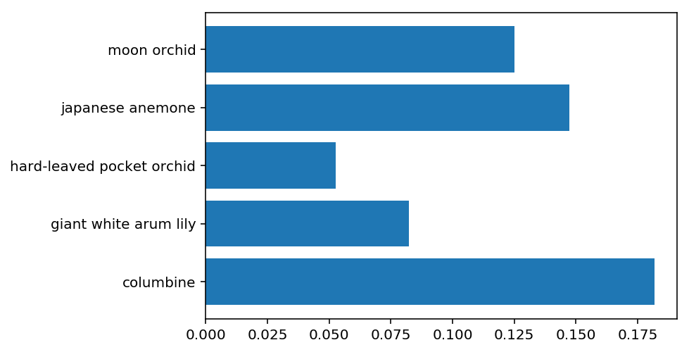
Sanity Checking
Even if the testing accuracy is high, it’s always good to check that there aren’t obvious bugs. Use matplotlib to plot the probabilities for the top 5 classes as a bar graph, along with the input image. It should look like this:
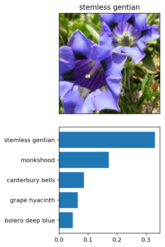
The class integer encoding can be converted to actual flower names with the cat_to_name.json file (should have been loaded earlier in the notebook). To show a PyTorch tensor as an image, use the imshow function defined above.
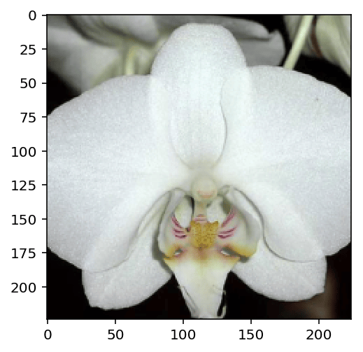
# Display an image along with the top 5 classes
# show sample photo
sample_img_dir = 'flowers/train/7/image_07203.jpg'
with Image.open(sample_img_dir) as im:
    image = process_image(im)
    imshow(image)
probs, classes = predict(sample_img_dir, imported_model)
Probabilities: tensor([[ 0.1818,  0.1474,  0.1250,  0.0822,  0.0527]])
Classes: ['84', '62', '7', '20', '2']
names = [cat_to_name[class_] for class_ in classes]
probs = probs.numpy()[0]
plt.barh(names, probs);
Skills &
Technologies
Libraries and technologies I have worked with in my projects. Proficiency ranges from advanced to familiar.